LM 33.3 Probability distributions Collection

33.3 Probability distributions

So far we've discussed random processes having only two possible outcomes: yes or no, win or lose, on or off. More generally, a random process could have a result that is a number. Some processes yield integers, as when you roll a die and get a result from one to six, but some are not restricted to whole numbers, for example the number of seconds that a uranium- $238$ $238$ atom will exist before undergoing radioactive decay.

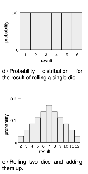
Consider a throw of a die. If the die is “honest,” then we expect all six values to be equally likely. Since all six probabilities must add up to $1$ $1$ , then probability of any particular value coming up must be $1$ $1$ / $6$ $6$ . We can summarize this in a graph, d. Areas under the curve can be interpreted as total probabilities. For instance, the area under the curve from $1$ $1$ to $3$ $3$ is $1 / 6 + 1 / 6 + 1 / 6 = 1 / 2$ $1"/"6+1"/"6+1"/"6=1"/"2$ , so the probability of getting a result from $1$ $1$ to $3$ $3$ is $1$ $1$ / $2$ $2$ . The function shown on the graph is called the probability distribution.

Figure e shows the probabilities of various results obtained by rolling two dice and adding them together, as in the game of craps. The probabilities are not all the same. There is a small probability of getting a two, for example, because there is only one way to do it, by rolling a one and then another one. The probability of rolling a seven is high because there are six different ways to do it: $1 + 6$ $1+6$ , $2 + 5$ $2+5$ , etc.

If the number of possible outcomes is large but finite, for example the number of hairs on a dog, the graph would start to look like a smooth curve rather than a ziggurat.

What about probability distributions for random numbers that are not integers? We can no longer make a graph with probability on the $y$ $y$ axis, because the probability of getting a given exact number is typically zero. For instance, there is zero probability that a radioactive atom will last for exactly $3$ $3$ seconds, since there are infinitely many possible results that are close to $3$ $3$ but not exactly $3$ $3$ , for example $2.999999999999999996876876587658465436$ $2.999999999999999996876876587658465436$ . It doesn't usually make sense, therefore, to talk about the probability of a single numerical result, but it does make sense to talk about the probability of a certain range of results. For instance, the probability that an atom will last more than $3$ $3$ and less than $4$ $4$ seconds is a perfectly reasonable thing to discuss. We can still summarize the probability information on a graph, and we can still interpret areas under the curve as probabilities.

But the $y$ $y$ axis can no longer be a unitless probability scale. In radioactive decay, for example, we want the $x$ $x$ axis to have units of time, and we want areas under the curve to be unitless probabilities. The area of a single square on the graph paper is then

$(unitless area of a square) = (width of square with time units) \times (height of square)$ $("unitless area of a square")=("width of square with time units")×("height of square")$ .

If the units are to cancel out, then the height of the square must evidently be a quantity with units of inverse time. In other words, the $y$ $y$ axis of the graph is to be interpreted as probability per unit time, not probability.

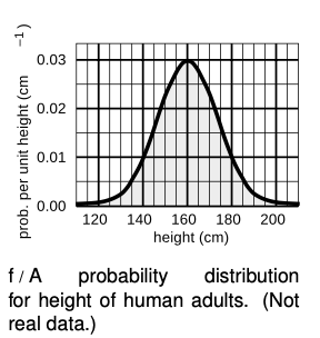
Figure f shows another example, a probability distribution for people's height. This kind of bell-shaped curve is quite common.

self-check:

Compare the number of people with heights in the range of $130 - 135$ $130-135$ cm to the number in the range $135 - 140$ $135-140$ .

(answer in the back of the PDF version of the book)

Example 1: Looking for tall basketball players

$\Rightarrow$ $=>$ A certain country with a large population wants to find very tall people to be on its Olympic basketball team and strike a blow against western imperialism. Out of a pool of $10^{8}$ $10^8$ people who are the right age and gender, how many are they likely to find who are over $225 c m$ $225 cm$ ( $7$ $7$ feet $4$ $4$ inches) in height? Figure g gives a close-up of the “tail” of the distribution shown previously in figure f.

$\Rightarrow$ $=>$ The shaded area under the curve represents the probability that a given person is tall enough. Each rectangle represents a probability of $2 \times 10^{- 7} c m^{- 1} \times 1 c m = 2 \times 10^{- 8}$ $2×10^(-7) cm^(-1)×1 cm=2×10^(-8)$ . There are about $35$ $35$ rectangles covered by the shaded area, so the probability of having a height greater than $225 c m$ $225 cm$ is $7 \times 10^{- 7}$ $7×10^(-7)$ , or just under one in a million. Using the rule for calculating averages, the average, or expected number of people this tall is $(10^{8}) \times (7 \times 10^{- 7}) = 70$ $(10^8)×(7×10^(-7))=70$ .

Average and width of a probability distribution

If the next Martian you meet asks you, “How tall is an adult human?,” you will probably reply with a statement about the average human height, such as “Oh, about $5$ $5$ feet $6$ $6$ inches.” If you wanted to explain a little more, you could say, “But that's only an average. Most people are somewhere between $5$ $5$ feet and $6$ $6$ feet tall.” Without bothering to draw the relevant bell curve for your new extraterrestrial acquaintance, you've summarized the relevant information by giving an average and a typical range of variation.

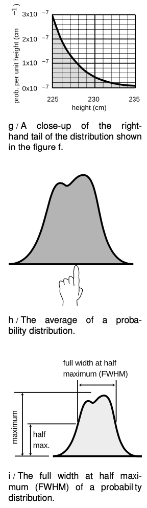
The average of a probability distribution can be defined geometrically as the horizontal position at which it could be balanced if it was constructed out of cardboard, h. A convenient numerical measure of the amount of variation about the average, or amount of uncertainty, is the full width at half maximum, or FWHM, defined in figure g. (The FWHM was introduced on p. 469.)

A great deal more could be said about this topic, and indeed an introductory statistics course could spend months on ways of defining the center and width of a distribution. Rather than force-feeding you on mathematical detail or techniques for calculating these things, it is perhaps more relevant to point out simply that there are various ways of defining them, and to inoculate you against the misuse of certain definitions.

The average is not the only possible way to say what is a typical value for a quantity that can vary randomly; another possible definition is the median, defined as the value that is exceeded with $50 %$ $50%$ probability. When discussing incomes of people living in a certain town, the average could be very misleading, since it can be affected massively if a single resident of the town is Bill Gates. Nor is the FWHM the only possible way of stating the amount of random variation; another possible way of measuring it is the standard deviation (defined as the square root of the average squared deviation from the average value).

33.3 Probability distributions by Benjamin Crowell, Light and Matter licensed under the Creative Commons Attribution-ShareAlike license.

LM 33.3 Probability distributions Collection

33.3 Probability distributions

Example 1: Looking for tall basketball players

Average and width of a probability distribution

This Collection is empty