Physics: Motion and Acceleration

vCalc Reviewed

Last modified by

WilliamC

Sep 29, 2022, 12:49:54 AM

Created by

MichaelBartmess

Dec 22, 2014, 5:56:27 AM

Position & Velocity

Acceleration

Constants of Speed

Kinematics Definition

Mechanics is a branch of physics that describes the behavior of physical bodies. The science of mechanics examines the forces and motions of these bodies and any effects these bodies may in turn exert on their environment.

Kinematics is a sub-discipline of mechanics which describes the motion of points, objects, and systems of objects while ignoring the causes of motion. In other words, Kinematics does not describe forces, it only describes models of displacement, velocity, and acceleration.

Position Vectors

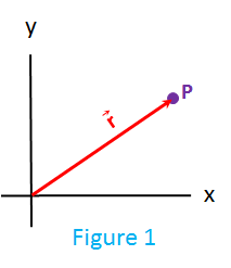
To describe motion we must first be able to describe position. In the Euclidean plane^[¹^]we can describe the position of a point or particle, P, using a position vector, `vecr`. Basically, the vector, `vecr`, has it's starting end at the origin of the Euclidean plane's x/y coordinates and extends from there to the point, P. A vector described like this can point to any position in the Euclidean x-y plane.

In the image of Figure 1, P resides in the quadrant of the Euclidean plane where both x and y are positive. The two dimensional position vector can point to any position in the Euclidean plane, so can point to positions in any of the four x-y quadrants.

A position vector can be further represented in Euclidean three-space with a three component position vector^[²^] that can be written as `vecr = xhati + yhatj + zhatk`. The x and y components of this three dimensional position vector might be represented as shown in Figure 1, with the additional z-component coming out of the page. If the z-component coming out of the page were zero, in other words `vecr = xhati + yhatj + 0hatk`, the two dimension position vector and the three dimensional position vector would be identical and as shown in Figure 1.

Magnitude of Position

If you know the individual components of the three-dimensional position vector (`r_x, r_y, r_z`) you can compute the magnitude of the position using this calculator's button labeled Magnitude of Position. This represented in component notation as:

`|vecr| = sqrt (r_x^2 + r_y^2 +r_z^2)` ^[7]

A two-dimensional version of the same equation, representing the magnitude of the position vector in the Euclidean plane only is given by:

`|vecr| = sqrt (r_x^2 + r_y^2 )`

Velocity Vectors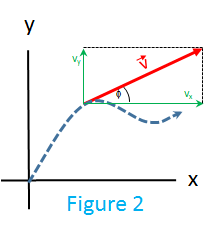

Velocity, as well as position, can be represented as a vector. We can represent the velocity of a particle, P, with any vector in the Euclidean plane as `vecv = v_xhati + v_yhatj`. In this representation, `v_x` and `v_y` are the x and y components of vector `vecv` as shown in Figure 2.

Average Velocity

The average velocity vector^[³^] can be represented as the ratio of the change in position to the change in time and can be shown as:

`vecv_"Avg"` = `(Deltavecr)/(Deltat)`

`|vecv_"Avg"|`^[3] = `(|Deltavecr|)/(Deltat) = |vecr_2 - vecr_1| / (t_2 - t_1)`

You can play with the inputs of the velocity vector in this calculator using the "Average Velocity" button. Try it out.

Instantaneous Velocity

The instantaneous velocity vector is the limit as the time denominator and the displacement of the the average velocity vector, `v_"Avg"`, goes to zero:

`v_"Inst"`^[⁴^] = `lim_(t->0) (|Deltavecr|)/(Deltat)`

The magnitude of this instantaneous velocity vector, `v_"Inst"`, at any instant is the speed of the particle. It is also important to note that the instantaneous velocity vector at any point in time is always tangent to the particle's path at that time point.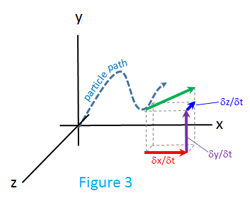 /attachments/44c60b61-899f-11e4-a9fb-bc764e2038f2/Velocity components 3D.png

To use the three-dimensional velocity vector, `vecv` to describe the instantaneous velocity of a particle or point, we often decompose (see Figure 3) the instantaneous velocity vector into it's constituent Euclidean components^[⁵^]:

`v_x = (dx)/(dt)`
`v_y = (dy)/(dt)`
`v_z = (dz)/(dt)`

This composition of the velocity vector, `vecv`, can be seen to be the derivative of the position vector, `vecr`, mentioned above:

`vecv = (dvecr)/(dt)`

and this in a component representation is:

`vecv = (dx)/(dt)hati + (dy)/(dt)hatj +(dz)/(dt)hatk` ^[⁶^]

Magnitude of Velocity

If you know the individual components of the velocity vector (`v_x, v_y, v_z`) you can compute the magnitude of the velocity using this calculator's button labeled Magnitude of Velocity. This represented in component notation as:

`|vecv| = sqrt (v_x^2 + v_y^2 +v_z^2)` ^[⁷^]

A two-dimensional version of the same equation, representing the magnitude of the velocity vector in the Euclidean plane only is given by:

`|vecv| = sqrt (v_x^2 + v_y^2 )`

Angle of the Velocity Vector

And in that two dimensional representation it is easy to see that the angle of the vector^[⁸^] relative to the x-axis is shown by the Pythagorean theorem to be `phi` in Figure 2. See also this calculator's button labeled Angle of the Vector (`v_y, v_x`):

`tan(theta) = v_y/v_x`

From the same look at the Pythagorean right angle relationship of `v_y` and `v_x`, we get the ability to calculate the angle of the velocity vector using the combination of the magnitude and the x-component (see calculator buttons labeled: Angle of the Vector (`|vecv|, v_x`) and Angle of the Vector (`|vecv|, v_y`)/

Velocity Constants

On this calculator you will find buttons for the Max velocity, that is the speed of light in a vacuum, along with the speed of sound provided in both English and metric units.

Acceleration Vectors

Average Acceleration

Analogous to the representation of the average velocity vector above, the average acceleration vector can be computed by the calculator button labeled Acceleration[`Deltav, Deltat`] and represented as:

`veca_"Avg"` = `(Deltavecv)/(Deltat)`

`|veca_"Avg"|` = `(|Deltavecv|)/(Deltat) = |vecv_2 - vecv_1| / (t_2 - t_1)` ^[⁹^]

The average acceleration vector, `a_"Avg"`, can be viewed as the vector subtraction of `vecv_2 - vecv_1`, as shown in Figure 4. The components of the average acceleration vector can also be decomposed into x and y components, so that:

`veca_"Avg -x"` = `(v_"2-x" - v_"1-x")`/ `(t_2 - t_1`)

Instantaneous Acceleration

The instantaneous acceleration vector is the limit as the `Deltat` denominator and the change in velocity, `Deltavecv`, of the the average acceleration vector, `a_"Avg"`, goes to zero:

`veca`^[¹⁰^] = `lim_(t->0) (|Deltavecv|)/(Deltat)`

As the `Deltavecv` and `Deltat` go to zero, the tangent points of the two velocity vectors, `vecv_1` and `vecv_2` approach the instantaneous rate of change of acceleration. The velocity vector, `vecv`, is tangent to the path of the particle and the instantaneous acceleration vector points to the concave side of the path of the particle.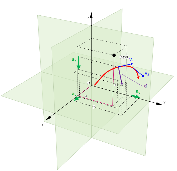 /attachments/44c60b61-899f-11e4-a9fb-bc764e2038f2/Acceleration components.png

Analogous to the composition of the instantaneous velocity vector, we can decompose the instantaneous acceleration vector into it's constituent Euclidean components^[¹¹^]:

`a_x = (dv_x)/(dt)`
`a_y = (dv_y)/(dt)`
`a_z = (dv_z)/(dt)`

This composition of the acceleration vector, `veca`, can be seen to be the derivative of the velocity vector, `vecv`, mentioned above:

`veca = (dvecv)/(dt)`

and this in a component representation is:

`veca = (dv_x)/(dt)hati + (dv_y)/(dt)hatj +(dv_z)/(dt)hatk` ^[¹²^]

or as the second derivative:

`veca = (d^2x)/(dt^2)hati + (d^2y)/(dt^2)hatj +(d^2z)/(dt^2)hatk` ^[¹³^]

Components of Acceleration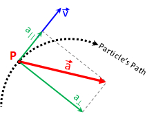

In addition to decomposing the acceleration vector into x, y and z components, parallel to the x, y and z axes of the Euclidean plane^[¹⁴^], there is a very useful decomposition of the acceleration vector in which the components parallel and perpendicular to the tangent at the point P are represented as `a"||"` and `a_"perp"`. The component `a"||"` is parallel to the velocity vector, `vecv`, making the `a_"perp"` component normal to the velocity vector, `vecv`.