LM 3_5 The area under the velocity-time graph Collection

3.5 The area under the velocity-time graph by Benjamin Crowell, Light and Matter  licensed under the Creative Commons Attribution-ShareAlike license.

3.5 The area under the velocity-time graph

A natural question to ask about falling objects is how fast they fall, but Galileo showed that the question has no answer. The physical law that he discovered connects a cause (the attraction of the planet Earth's mass) to an effect, but the effect is predicted in terms of an acceleration rather than a velocity. In fact, no physical law predicts a definite velocity as a result of a specific phenomenon, because velocity cannot be measured in absolute terms, and only changes in velocity relate directly to physical phenomena.

The unfortunate thing about this situation is that the definitions of velocity and acceleration are stated in terms of the tangent-line technique, which lets you go from `x` to `v` to `a`, but not the other way around. Without a technique to go backwards from `a` to `v` to `x`, we cannot say anything quantitative, for instance, about the `x-t` graph of a falling object. Such a technique does exist, and I used it to make the `x-t` graphs in all the examples above.

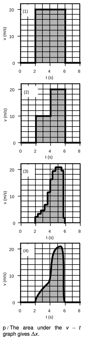First let's concentrate on how to get `x` information out of a `v-t` graph. In example p/1, an object moves at a speed of `20 m"/"s` for a period of 4.0 s. The distance covered is `Deltax=v•Deltat`=`(20 m"/"s)×(4.0 s)=80 m`. Notice that the quantities being multiplied are the width and the height of the shaded rectangle  or, strictly speaking, the time represented by its width and the velocity represented by its height. The distance of Δx = 80m  thus corresponds to the area of the shaded part of the graph.

The next step in sophistication is an example like p/2, where the object moves at a constant speed of `10 m"/"s` for two seconds, then for two seconds at a different constant speed of `20 m"/"s`. The shaded region can be split into a small rectangle on the left, with an area representing `Deltax=20 m`, and a taller one on the right, corresponding to another 40 m of motion. The total distance is thus 60 m, which corresponds to the total area under the graph.
  o / The area under the `v-t` graph gives Δx. 
An example like p/3 is now just a trivial generalization; there is simply a large number of skinny rectangular areas to add up. But notice that graph p/3 is quite a good approximation to the smooth curve p/4. Even though we have no formula for the area of a funny shape like p/4, we can approximate its area by dividing it up into smaller areas like rectangles, whose area is easier to calculate. If someone hands you a graph like p/4 and asks you to find the area under it, the simplest approach is just to count up the little rectangles on the underlying graph paper, making rough estimates of fractional rectangles as you go along.

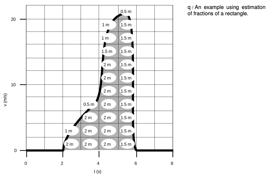
That's what I've done in figure q. Each rectangle on the graph paper is 1.0 s wide and `2 m"/"s` tall, so it represents 2 m. Adding up all the numbers gives `Deltax=41 m`. If you needed better accuracy, you could use graph paper with smaller rectangles.

It's important to realize that this technique gives you `Deltax`, not `x`. The `v-t` graph has no information about where the object was when it started.

The following are important points to keep in mind when applying this technique:

• If the range of `v` values on your graph does not extend down to zero, then you will get the wrong answer unless you compensate by adding in the area that is not shown.
• As in the example, one rectangle on the graph paper does not necessarily correspond to one meter of distance.
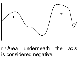
• Negative velocity values represent motion in the opposite direction, so as suggested by figure r, area under the `t` axis should be subtracted, i.e., counted as “negative area.”

• Since the result is a `Deltax` value, it only tells you `x_(after) - x_"before"`, which may be less than the actual distance traveled. For instance, the object could come back to its original position at the end, which would correspond to `x=0`, even though it had actually moved a nonzero distance.

Finally, note that one can find `v` from an `a-t` graph using an entirely analogous method. Each rectangle on the `a-t` graph represents a certain amount of velocity change.

Discussion Question

⇒ Roughly what would a pendulum's `v-t` graph look like? What would happen when you applied the area-under-the-curve technique to find the pendulum's `x` for a time period covering many swings?

3.5 The area under the velocity-time graph by Benjamin Crowell, Light and Matter  licensed under the Creative Commons Attribution-ShareAlike license.